Zero Sections of Vector Bundles

This post walks through some interesting results on real and complex line bundles, leading up to a discussion of the Euler class for complex line bundles, which characterizes their zero sections. Briefly, a complex line bundle is a topological object which generalizes the space of complex-valued functions defined on some domain. The "sections" of the complex line bundle locally behave like complex functions, but their global structure must obey certain constraints. In particular, their zero sets must belong to a particular topological class, prescribed by the line bundle's Euler class. Here, I detail some concrete, low-dimensional examples that I found useful for thinking about these topics.

Prelude: vector fields on the sphere

The hairy ball theorem famously states that any continuous tangent vector field on the sphere must have a zero, i.e. there must be some point on the sphere where the vector field is zero. Indeed, this result can be strengthened to tell us about the required number of zeros: the sum of the indices of the zeros must equal the Euler characteristic of the domain. In particular, since the sphere has Euler characteristic 2, any vector field on the sphere must have at least one zero.

On the other hand, it's very easy to define an \(\RR^2\)-valued function on the sphere with no zeros: even the constant function \(f(x) = (1, 0)\) works. Although tangent vector fields and \(\RR^2\)-valued functions sound very similar when you first learn about them—and indeed, any tangent vector field can locally be written as an \(\RR^2\)-valued function—their global behavior is quite different. And in particular, the zero sets of tangent vector fields must obey delicate constraints which vector-valued functions are free to ignore. To get a better understanding of what's going on here, it may help to step down a dimension, and look at real-valued functions on the one dimensional sphere, i.e. the circle.

The circle

Let's start by looking at the circle \(S^1 := \{ x \in \RR^2 \;:\; \|x\| = 1\}\), and considering real-valued functions \(f : S^1 \to \RR^1\). We can identify these functions with functions \(f : [0, 1] \to \RR^1\) defined on the unit interval subject to the constraint that \(f(0) = f(1)\). And the nice thing about moving down to one dimension is that these functions are very easy to visualize. We can graph these functions over the unit interval, and we can even draw these graphs on the cylinder to emphasize the constraint that \(f(0) = f(1)\).

In one dimension, though, tangent vector fields are a lot simpler. It's easy to construct non-vanishing vector fields on the circle—for instance, you can take the vector field that always points counterclockwise.

A nonvanishing vector field on the circle

Indeed, tangent vector fields on the circle are in one-to-one correspondence with real-valued functions on the circle. So they don't really help us understand what's going on with the hairy ball theorem in 2D. We will have to look elsewhere.

Twisted functions on the circle

The key is to consider the picture of graphs drawn on the cylinder. We can introduce a twist and consider "graphs" which are drawn on the Möbius strip instead.

While this construction may sound kind of arbitrary, but this notion of generalized graphs ends up being surprisingly useful throughout math and physics. Although these graphs no longer represent continuous functions defined on the circle, they can still be written using functions \(f : [0, 1] \to \RR^1\) defined on the unit interval. The difference is that thanks to the twist in the Möbius strip, we have a new compatibility condition: this time, we require that \(f(0) = - f(1)\). For now, I will call these functions "twisted functions," since their graphs are continuous on the twisted Möbius strip¹. And importantly, our new compatibility condition forces all of our twisted functions to have at least one zero! They must pass zero as they go from negative to positive (or vice versa). Using this Möbius strip example, we can now return to two-dimensional surfaces and find some more interesting examples of twisted functions.

Twisted functions on the torus

Now we will move back to the setting of two-dimensional surfaces, but we will continue to think about real-valued functions to start with. Consider the torus \(T^2\), and a real-valued function \(f : T^2 \to \RR\). We can draw the graph of \(f\) as a two-dimensional surfaces living inside of the three-dimensional thickened torus \(T^2 \times I\).

Any loop \(S^1 \subset T^2\) in the torus becomes a topological cylinder (or equivalently, an annulus) in the thickened cylinder. What happens if we replace some of those cylinders with Möbius strips instead?

For instance, suppose we replace the cylinder over each of the longitudinal loops with a Möbius strip. The figure below shows the resulting twisted thickened torus, with several of the component Möbius strips highlighted.

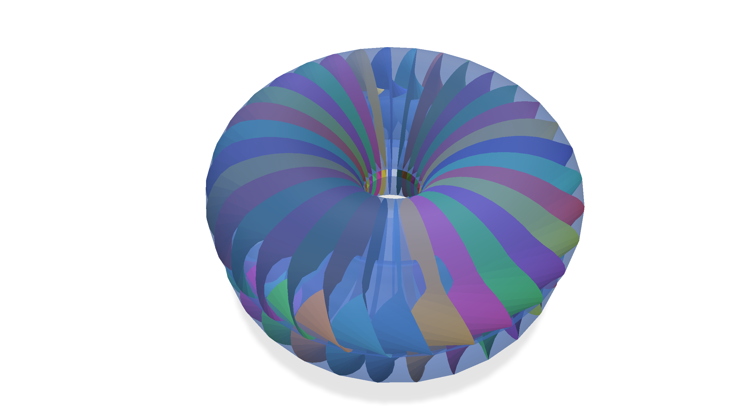
We saw above that a twisted function drawn on the Möbius strip must have a zero somewhere. This torus has a Möbius strip on each of its lateral loops, so a twisted function defined on the torus must have a zero on each lateral loop. That means that the zero set of the twisted function must be a curve which wraps one or more times around the torus!

And of course, the direction that the zero set wraps around the torus was determined by the fact that we chose to put Möbius strips over the longitudinal loops. If we twisted the thickened torus in other ways, then we could force the zero sets of our twisted functions to follow different paths along the torus.

The homological perspective

In general, if we start with an oriented \(n\)-dimensional manifold \(M\), and we look at the zero set \(S\) of a single real function, we expect \(S\) to be an \((n-1)\)-dimensional submanifold. In this case, the zero set defines an \((n-1)\)-dimensional homology class \([S] \in H_{n-1}(M)\). By Poincaré duality, we can identify homology classes \(S \in H_{n-1}(M)\) with one-dimensional cohomology classes \([\eta] \in H^1(M)\). In the language of differential forms, the Poincaré dual of a homology class \(S\) is a harmonic 1-form \(\eta\) with flux 1 through \(S\) and zero flux through all other homology classes of submanifolds.

All this is pretty abstract, so it may help to revisit our torus example. In that case, we saw that our zero set \(S\) wrapped horizontally around the torus. The dual 1-form \(\eta\) should thus wind around the torus in the longitudinal direction—exactly the way that we glued our Möbius strips.

Left: the integral curves of the 1-form \(\eta\) describe the loops that we placed Möbius strips on. Right: the zero set \(S\) of our twisted function is the dual of the 1-form \(\eta\).

Unfortunately, this twisting trick doesn't let us prescribe the exact homology class \([S] \in H_{n-1}(M)\) of the zero set. Going back to the circle example, we can start from a cylinder and add a single twist to ensure that our zero set contains at least one point. But we cannot then add a second twist to ensure that the zero set contains at least two points: topologically speaking, adding that second twist just brings us back from the Möbius strip to the cylinder again! In general, adding these twists only allows us to control the mod-2 homology class of the zero set, \([S] \in H_{n-1}(M;\mathbb{Z}/2\mathbb{Z})\). But amazingly, this restriction disappears in the complex case!

Mathematical terminology: vector bundles

But before proceeding, it will help to lay out a little more mathematical terminology that I've been avoiding so far. When we have a domain \(M\) and a vector-valued function \(f : M \to \RR^d\), we can draw its graph in the product space \(M \times \RR^d\). For each point \(x \in M\) this product space contains a separate copy of \(\RR^d\), which we denote by \(\RR^d_x\). And all of these copies of \(\RR^d\) fit together in a continuous way just as we built a cylinder earlier by gluing together a bunch of lines over a circle.

The product space \(M \times \RR^d\) is an example of a vector bundle, a collection of vector spaces "bundled up" over the points of some base space. Locally, vector bundles look like simple product spaces, and in particular, they still contain a separate copy of \(\RR_x^d\) for each point \(x\) in the base space. But globally they can behave quite differently. For instance, any small patch of the Möbius strip looks identically to a small patch on the cylinder, but we already saw that the Möbius strip has different global properties.

Another classic example of a vector bundle is the tangent bundle \(TM\) of a manifold \(M\). If \(M\) is an \(n\)-dimensional manifold, then \(TM\) contains an \(n\)-dimensional vector space \(T_xM\) associated to each point \(x \in M\). In general, the tangent space \(TM\) is not equal to the simple product space \(M \times \RR^n\), leading to results like the hairy ball theorem for the two-dimensional sphere which we saw earlier.

Vector bundles are often used to define spaces of generalized functions, like the graphs that we drew on the Möbius strip, or tangent vector fields on a manifold. Whereas an ordinary vector-valued function takes in a point \(x\) in the domain and returns a vector \(f(x) \in \RR^d\), our twisted functions on a vector bundle will instead return a vector \(f(x) \in \RR^d_x\) living in the special vector space associated to point \(x\). These twisted functions are usually referred to as sections (or cross-sections) of the vector bundle.

The complex case

If we look at the zero set \(S\) of a single complex function on an \(n\)-dimensional manifold \(M\), then we generically expect \(S\) to be an \((n-2)\)-dimensional submanifold, defining a homology class \(S \in H_{n-2}(M)\). And again, Poincaré duality allows us to identify \(S\) with its dual cohomology class \(\eta \in H^2(M)\). But this time, unlike in the real case, we can use special twists to force \(S\) to lie in any homology class of \(H_{n-2}(M)\) that we like: picking twists gives us complete control over the topology of the zero sets.

Another way of saying this is that the cohomology class \(\eta\) is determined by the topological structure of the vector bundle that we build over \(M\). Since our vector spaces are always the complex line \(\CC^1\), these vector bundles are referred to as complex line bundles. And the cohomology class \(\eta \in H^2(M)\) is known as the first Chern class, or the Euler class, of the line bundle.

These sorts of facts about complex line bundles, sections, and Chern classes are usually proved using pretty abstract arguments involving the classifying space \(\CC P^\infty\), which provides an alternative representation of complex line bundles. Instead of taking that path, I will work through some details of the complex analogue of the Möbius strip. We won't prove the general versions of these results, but I found the example helpful for building intuition.

Unfortunately, even the simplest complex line bundles are quite complicated. In the real case, we started with a one-dimensional circle, and built a real line bundle by gluing on one-dimensional lines to obtain a two-dimensional Möbius strip. In the complex case, we will start with the two-dimensional sphere \(S^2\) and build a complex line bundle by gluing on two-dimensional complex planes to obtain an object with four real dimensions (or two complex dimensions if you want to go all in with complex thinking). So it will be a lot harder to draw pictures.

Starting with the sphere

My discussion here follows the treatment in Chapter 1 of Hatcher's book on vector bundles. First, Hatcher notes that we can build a complex line bundle on the sphere by the following construction: we think of the sphere \(S^2\) as the union of the northern hemisphere \(D^+\) and the southern hemisphere \(D^-\), which intersect exactly along the equator \(D^+ \cap D^- = S^1\).

On each hemisphere, we build our complex line bundle as the product \(D^\pm \times \CC\), and we glue together these two halves using a "clutching map" \(f : S^1 \to \CC \setminus 0\) which tells us how the vector spaces at each point of the equator in northern hemisphere should be rotated and scaled before gluing them to the corresponding vector spaces in the southern hemisphere. This construction is still pretty opaque, so we can start by considering how it applies to the real case of the Möbius strip again.

Clutching maps for the Möbius strip

We start by decomposing the circle into northern and southern intervals \(I^\pm\), which intersect at the equator \(S^0\), consisting of a pair of opposite points. Once we thicken each hemisphere separately, we get a pair of strips \(I^\pm \times I\), and the only remaining question is how to glue them together again.

This gluing is determined by a clutching map \(f : S^0 \to \RR \setminus 0\). The map \(f\) gives a nonzero number for the left and right points of the equator; for each side, we glue the ends of our strips directly if the number is positive and glue them with a twist if the number is negative.

The fact that we only need the sign of \(f\), rather than the precise value, reflects the fact the vector bundle we get from this clutching map construction depends only on the homotopy class of the clutching map. Furthermore, we can restrict our attention to basepoint-preserving maps (which always send the left endpoint of \(S^0\) to \(1\)), yielding only two homotopy classes of basepoint-preserving maps: those which send the left point to a positive number, and those which send the left point to a negative number.

So the two real line bundles over the circle that we saw earlier—the cylinder and the Möbius strip—are the only two possibilities, and correspond exactly to the two homotopy classes of basepoint-preserving maps from \(S^0 \to \RR\setminus 0\).

Complex line bundles on the sphere

The situation with complex line bundles on the two-dimensional sphere \(S^2\) is exactly analogous. Except this time, our clutching functions are maps \(f : S^1 \to \CC \setminus 0\). Any such map is homotopic to a map \(g : S^1 \to S^1\) (e.g. the normalization of \(f\)), so we get a complex line bundle on the sphere for each homotopy class of maps from \(S^1\) to itself. The homotopy classes of maps from \(S^1\) to \(S^1\) are precisely the loops in \(\pi_1(S^1) \cong \ZZ\), so we have one complex line bundle over the sphere for each integer.

That's a good sign: we wanted to rig up our complex line bundles to force the zero sets to lie in a particular homology class in \(H_0(S^2) \cong \ZZ\). So at least we have the right number of complex line bundles. Now we will look more closely at how the clutching map construction determines the zeros of a section of our complex line bundle.

Suppose we start with a complex line bundle on the sphere, and a section \(\Gamma\). We can think of the hemisphere decomposition that we've been using as a pair of charts for the vector bundle, with the clutching map acting as our transition function between the charts. But, of course, it's not important that our hemispheres cut the sphere exactly in half. Topologically speaking, we can pick any two disks that cover the sphere and meet along a circle. So we're free to make the hemisphere \(D^+\) huge, covering almost all of the sphere, and the other hemisphere \(D^-\) tiny.

Our decomposition of the sphere into hemispheres need not cut the sphere exactly in half: we can pick any decomposition into two topological disks.

If we put \(D^-\) in a place where our section \(\Gamma\) is nonzero, then we can change \(\Gamma\) by a small homotopy to make it constant in \(D^-\) without changing its zero set. Now, all of the interesting behavior of \(\Gamma\) occurs over \(D^+\), where our charts allow us to write \(\Gamma\) as an honest complex function \(\Gamma : D^+ \to \CC\). However, \(\Gamma\) cannot be any arbitrary complex function: on the boundary of \(D^+\), it must agree with the value from \(D^-\). To be precise, for each point \(x \in \partial D^+\), the value \(\Gamma(x)\) (written in the \(D^+\) chart) must equal \(f(x)\) times the constant value of \(\Gamma\) on \(D^-\) (written in the \(D^-\) chart).

Up to multiplication by a nonzero complex constant (which does not change the zeros of \(\Gamma\)), this means that we have prescribed nonzero vectors for \(\Gamma(x) \in \RR^2\) on \(S^1 = \partial D^+\), and \(\Gamma\) continuously interpolates those values into the interior. The homotopy class of our clutching map \(f\) determines the turning number of \(\Gamma\) along the boundary \(\partial D^+\), i.e. the total number of rotations that \(\Gamma\) makes as you walk along the boundary. Now, the standard Poincaré-Hopf theorem tells us that the sum of the indices of the zero set of our vector field inside the disk is precisely equal to this turning number!

The tangent bundle of the sphere

Finally, we'll take a look at how everything works out for the familiar tangent bundle \(TS^2\) of the two-dimensional sphere. This calculation is taken from Example 1.9 of Hatcher's book on vector bundles.

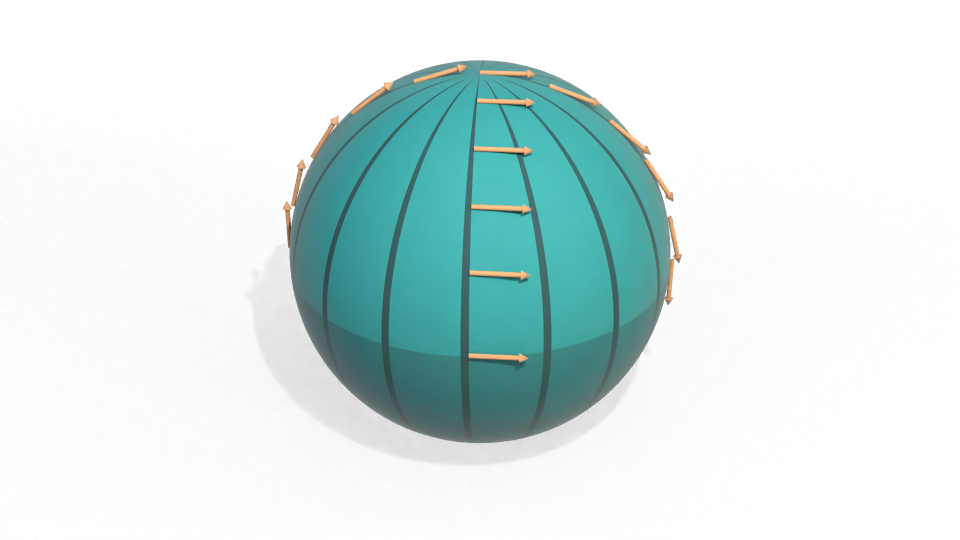
To construct a clutching map for \(TS^2\), we first decompose \(S^2\) into its northern and southern hemispheres in the usual way, with the equator \(S^1\) running around the middle of the sphere. We define our chart on the northern hemisphere by picking an arbitrary vector at the north pole and parallel transporting it along lines of longitude to all other points in the northern hemisphere. This defines the \(x\)-axis of our tangent basis at each point, and we get \(y\)-axes by rotating these vectors 90 degrees counterclockwise about the normal vector to each point.

Some of our basis vectors in the northern hemisphere.

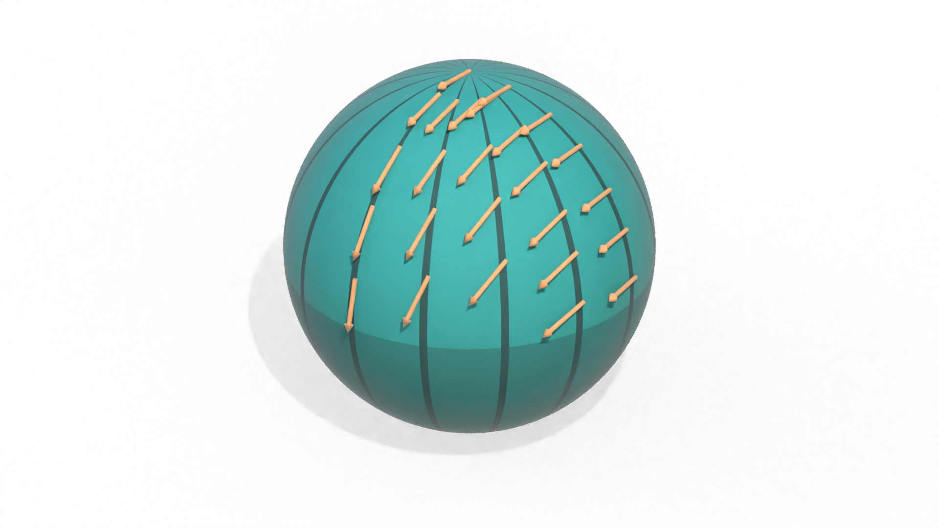
This choice of bases allows us to write any vector field in the northern hemisphere as an element of \(D^+ \times \RR^2\). We can similarly define tangent bases for points in the southern hemisphere by parallel transporting a vector in the same direction form the south pole. Now, we just need to work out the clutching map for this choice of charts on the northern and southern hemispheres. The clutching map should tell us the relative angle between the two \(x\)-axis vectors which we obtain at points on the equator.

Note that if we start off with the vector \((1, 0, 0)\) at the north and south poles, then our vectors at the equator point in the same direction at the \(\pm y\) ends of the sphere, and point in opposite directions at the \(\pm x\) points of the sphere.

In general, if we parameterize the points on the equator by their angle \(\theta\) with the \(+y\) point \((0, 1, 0)\), the angle at which our vectors meet is given by \(f(\theta) = 2\theta\). Hence, the homotopy class \([f]\) of our clutching map corresponds to the element \(2 \in \pi_1(S^1) \simeq \ZZ\). As we saw earlier, this means that the sum of the indices of the zeros of a section must be \(2\). Which is exactly the result guaranteed by the usual Poincaré-Hopf theorem.

Footnotes

1. Formally, these "twisted functions" are called "sections of a vector bundle," but we won't need this general language until later.